
View Code
knitr::opts_chunk$set(echo = TRUE)
library(tidyverse)
library(here)
library(janitor)
library(readxl)
library(sf)
library(USAboundaries)
library(scales)
library(ggthemes)
library(gghighlight)
library(ggnewscale)The data in this portfolio is available from the United States Geological Survey for years 1950-2015.
knitr::opts_chunk$set(echo = TRUE)
library(tidyverse)
library(here)
library(janitor)
library(readxl)
library(sf)
library(USAboundaries)
library(scales)
library(ggthemes)
library(gghighlight)
library(ggnewscale)#Read 1950 data,skip rows, read sheets and join, clean names, turn to numeric,
#and filter out NA
d_wu_1950 <- lapply(excel_sheets(here("data/water_use/us1950.xlsx")),
function(x) read_excel(here("data/water_use/us1950.xlsx"), skip = 3, sheet = x)) %>%
reduce(left_join, by = "Area") %>%
clean_names() %>%
mutate(across(c(1:9), as.numeric)) %>%
select(-contains("note_")) %>%
replace(is.na(.), 0)
#Read 1955 data,skip rows, read sheets and join, clean names, turn to numeric,
#and filter out NA
d_wu_1955 <- lapply(excel_sheets(here("data/water_use/us1955.xlsx")),
function(x) read_excel(here("data/water_use/us1955.xlsx"), skip = 3, sheet = x)) %>%
reduce(left_join, by = "Area") %>%
clean_names() %>%
mutate(across(c(1:10), as.numeric)) %>%
select(-contains("note_")) %>%
replace(is.na(.), 0)
#Read 1960 data,skip rows, read sheets and join, clean names, turn to numeric,
#and filter out NA
d_wu_1960 <- lapply(excel_sheets(here("data/water_use/us1960.xlsx")),
function(x) read_excel(here("data/water_use/us1960.xlsx"), skip = 3, sheet = x)) %>%
reduce(left_join, by = "Area") %>%
clean_names() %>%
mutate(across(c(1:35), as.numeric)) %>%
replace(is.na(.), 0)
#Read 1965 data,skip rows, read sheets and join, clean names, turn to numeric,
#and filter out NA
d_wu_1965 <- lapply(excel_sheets(here("data/water_use/us1965.xlsx")),
function(x) read_excel(here("data/water_use/us1965.xlsx"), skip = 3, sheet = x)) %>%
reduce(left_join, by = "Area") %>%
clean_names() %>%
mutate(across(c(1:33), as.numeric)) %>%
replace(is.na(.), 0)
#Read 1970 data,skip rows, read sheets and join, clean names, turn to numeric,
#and filter out NA
d_wu_1970 <- lapply(excel_sheets(here("data/water_use/us1970.xlsx")),
function(x) read_excel(here("data/water_use/us1970.xlsx"), skip = 3, sheet = x)) %>%
reduce(left_join, by = "Area") %>%
clean_names() %>%
mutate(across(c(1:34), as.numeric)) %>%
replace(is.na(.), 0)
#Read 1975 data,skip rows, read sheets and join, clean names, turn to numeric,
#and filter out NA
d_wu_1975 <- lapply(excel_sheets(here("data/water_use/us1975.xlsx")),
function(x) read_excel(here("data/water_use/us1975.xlsx"), skip = 3, sheet = x)) %>%
reduce(left_join, by = "Area") %>%
clean_names() %>%
mutate(across(c(1:34), as.numeric)) %>%
replace(is.na(.), 0)
#Read 1980 data,skip rows, read sheets and join, clean names, turn to numeric,
#and filter out NA
d_wu_1980 <- lapply(excel_sheets(here("data/water_use/us1980.xlsx")),
function(x) read_excel(here("data/water_use/us1980.xlsx"), skip = 3, sheet = x)) %>%
reduce(left_join, by = "Area") %>%
clean_names() %>%
mutate(across(c(1:34), as.numeric)) %>%
replace(is.na(.), 0)
#Read 1985 data, clean names, turn to numeric, and filter out NA
d_wu_1985 <- read_tsv(here("data/water_use/us1985.txt")) %>%
clean_names() %>%
mutate(across(c(4:163), as.numeric)) %>%
replace(is.na(.), 0)
#Read 1990 data, clean names, turn to numeric, filter NA in state,
#and replace NA with 0
d_wu_1990 <- read_xls(here("data/water_use/us1990.xls")) %>%
clean_names() %>%
filter(state != "NA") %>%
mutate(across(c(4:163), as.numeric)) %>%
replace(is.na(.), 0)
#Read 1995 data, clean names, turn to numeric, filter NA in state,
#and replace NA with 0
d_wu_1995 <- read_xls(here("data/water_use/us1995.xls")) %>%
clean_names() %>%
filter(state != "NA") %>%
mutate_at((1), as.numeric) %>%
mutate(across(c(3:4), as.numeric)) %>%
mutate(across(c(6:252), as.numeric)) %>%
replace(is.na(.), 0)
#Read 2000 data, clean names, turn to numeric, filter NA in state,
#and replace NA with 0
d_wu_2000 <- read_xls(here("data/water_use/us2000.xls")) %>%
clean_names() %>%
filter(state != "NA") %>%
mutate(across(c(2:70), as.numeric)) %>%
replace(is.na(.), 0)
#Read 2005 data, clean names, turn to numeric, filter NA in state,
#and replace NA with 0
d_wu_2005 <- read_xls(here("data/water_use/us2005.xls")) %>%
clean_names() %>%
filter(state != "NA") %>%
mutate(across(c(2:4), as.numeric)) %>%
mutate(across(c(6:108), as.numeric)) %>%
replace(is.na(.), 0)
#Read 2010 data, clean names, turn to numeric, filter NA in state,
#and replace NA with 0
d_wu_2010 <- read_xlsx(here("data/water_use/us2010.xlsx")) %>%
clean_names() %>%
filter(state != "NA") %>%
mutate_at((2), as.numeric) %>%
mutate(across(c(4:117), as.numeric)) %>%
replace(is.na(.), 0)
#Read 2015 data, clean names, turn to numeric, filter NA in state,
#and replace NA with 0
d_wu_2015 <- read_xlsx(here("data/water_use/us2015.xlsx"), skip = 1) %>%
clean_names() %>%
filter(state != "NA") %>%
mutate_at((2), as.numeric) %>%
mutate(across(c(4:141), as.numeric)) %>%
replace(is.na(.), 0)#Assign d_wu_year to wu_year
#Create new columns (State, Public Supply, Irrigation, Rural, Industrial,
#Thermoelectric, and Year)
#Pivot longer to create "Sectors" and "Withdrawals" column
#1950
wu_1950 <- d_wu_1950 %>%
mutate(State = area,
"Public Supply" = ps_wgw_fr + ps_wsw_fr,
Irrigation = ir_wgw_fr + ir_wsw_fr,
Rural = NA,
Industrial = inpt_wgw_fr + inpt_wsw_fr,
Thermoelectric = NA,
Year = 1950) %>%
select(State, "Public Supply", Irrigation, Rural, Industrial, Thermoelectric, Year) %>%
pivot_longer(2:6, names_to = "Sectors", values_to = "Withdrawals")
#1955
wu_1955 <- d_wu_1955 %>%
mutate(State = area,
"Public Supply" = ps_wgw_fr + ps_wsw_fr,
Irrigation = ir_wgw_fr + ir_wsw_fr,
Rural = NA,
Industrial = inpt_wgw_fr + inpt_wsw_fr,
Thermoelectric = NA,
Year = 1955) %>%
select(State, "Public Supply", Irrigation, Rural, Industrial, Thermoelectric, Year) %>%
pivot_longer(2:6, names_to = "Sectors", values_to = "Withdrawals")
#1960
#Replace ir_wsw_fr and ir_wgw_fr with ir_w_fr_to (The two columns do not have any data)
wu_1960 <- d_wu_1960 %>%
mutate(State = area,
"Public Supply" = ps_wgw_fr + ps_wsw_fr,
Irrigation = ir_w_fr_to,
Rural = do_wgw_fr + do_wsw_fr + ls_wgw_fr + ls_wsw_fr,
Industrial = oi_wgw_fr + oi_wsw_fr,
Thermoelectric = pt_wgw_fr + pt_wsw_fr,
Year = 1960) %>%
select(State, "Public Supply", Irrigation, Rural, Industrial, Thermoelectric, Year) %>%
pivot_longer(2:6, names_to = "Sectors", values_to = "Withdrawals")
#1965
wu_1965 <- d_wu_1965 %>%
mutate(State = area,
"Public Supply" = ps_wgw_fr + ps_wsw_fr,
Irrigation = ir_wgw_fr + ir_wsw_fr,
Rural = do_wgw_fr + do_wsw_fr + ls_wgw_fr + ls_wsw_fr,
Industrial = oi_wgw_fr + oi_wsw_fr,
Thermoelectric = pt_wgw_fr + pt_wsw_fr,
Year = 1965) %>%
select(State, "Public Supply", Irrigation, Rural, Industrial, Thermoelectric, Year) %>%
pivot_longer(2:6, names_to = "Sectors", values_to = "Withdrawals")
#1970
wu_1970 <- d_wu_1970 %>%
mutate(State = area,
"Public Supply" = ps_wgw_fr + ps_wsw_fr,
Irrigation = ir_wgw_fr + ir_wsw_fr,
Rural = do_wgw_fr + do_wsw_fr + ls_wgw_fr + ls_wsw_fr,
Industrial = oi_wgw_fr + oi_wsw_fr,
Thermoelectric = pt_wgw_fr + pt_wsw_fr,
Year = 1970) %>%
select(State, "Public Supply", Irrigation, Rural, Industrial, Thermoelectric, Year) %>%
pivot_longer(2:6, names_to = "Sectors", values_to = "Withdrawals")
#1975
wu_1975 <- d_wu_1975 %>%
mutate(State = area,
"Public Supply" = ps_wgw_fr + ps_wsw_fr,
Irrigation = ir_wgw_fr + ir_wsw_fr,
Rural = do_wgw_fr + do_wsw_fr + ls_wgw_fr + ls_wsw_fr,
Industrial = oi_wgw_fr + oi_wsw_fr,
Thermoelectric = pt_wgw_fr + pt_wsw_fr,
Year = 1975) %>%
select(State, "Public Supply", Irrigation, Rural, Industrial, Thermoelectric, Year) %>%
pivot_longer(2:6, names_to = "Sectors", values_to = "Withdrawals")
#1980
wu_1980 <- d_wu_1980 %>%
mutate(State = area,
"Public Supply" = ps_wgw_fr + ps_wsw_fr,
Irrigation = ir_wgw_fr + ir_wsw_fr,
Rural = do_wgw_fr + do_wsw_fr + ls_wgw_fr + ls_wsw_fr,
Industrial = oi_wgw_fr + oi_wsw_fr,
Thermoelectric = pt_wgw_fr + pt_wsw_fr,
Year = 1980) %>%
select(State, "Public Supply", Irrigation, Rural, Industrial, Thermoelectric, Year) %>%
pivot_longer(2:6, names_to = "Sectors", values_to = "Withdrawals")
#From 1985 and on add the following:
#Group by state
#Add across columns 1:5
#Add "Year" column
#1985
wu_1985 <- d_wu_1985 %>%
mutate(State = scode,
"Public Supply" = ps_wgwfr + ps_wswfr,
Irrigation = ir_wgwfr + ir_wswfr,
Rural = do_ssgwf + do_ssswf + ls_gwtot + ls_swtot,
Industrial = in_wgwfr + in_wswfr + mi_wgwfr + mi_wswfr,
Thermoelectric = pt_wgwfr + pt_wswfr,
Year = 1985) %>%
select(State, "Public Supply", Irrigation, Rural, Industrial, Thermoelectric, Year) %>%
group_by(State) %>%
summarise(across(1:5, sum)) %>%
mutate(Year = 1985) %>%
pivot_longer(2:6, names_to = "Sectors", values_to = "Withdrawals")
#1990
wu_1990 <- d_wu_1990 %>%
mutate(State = scode,
"Public Supply" = ps_wgwfr + ps_wswfr,
Irrigation = ir_wgwfr + ir_wswfr,
Rural = do_ssgwf + do_ssswf + ls_gwtot + ls_swtot,
Industrial = in_wgwfr + in_wswfr + mi_wgwfr + mi_wswfr,
Thermoelectric = pt_wgwfr + pt_wswfr,
Year = 1990) %>%
select(State, "Public Supply", Irrigation, Rural, Industrial, Thermoelectric, Year) %>%
group_by(State) %>%
summarize(across(1:5, sum)) %>%
mutate(Year = 1990) %>%
pivot_longer(2:6, names_to = "Sectors", values_to = "Withdrawals")
#1995
wu_1995 <- d_wu_1995 %>%
mutate(State = state_code,
"Public Supply" = ps_wgw_fr + ps_wsw_fr,
Irrigation = ir_wgw_fr + ir_wsw_fr,
Rural = do_wgw_fr + do_wsw_fr + ls_wgw_fr + ls_wsw_fr,
Industrial = in_wgw_fr + in_wsw_fr + mi_wgw_fr + mi_wsw_fr,
Thermoelectric = pt_wgw_fr + pt_wsw_fr,
Year = 1995) %>%
select(State, "Public Supply", Irrigation, Rural, Industrial, Thermoelectric, Year) %>%
group_by(State) %>%
summarize(across(1:5, sum)) %>%
mutate(Year = 1995) %>%
pivot_longer(2:6, names_to = "Sectors", values_to = "Withdrawals")
#2000
wu_2000 <- d_wu_2000 %>%
mutate(State = statefips,
"Public Supply" = ps_wgw_fr + ps_wsw_fr, Irrigation = it_wgw_fr + it_wsw_fr,
Rural = do_wgw_fr + do_wsw_fr + ls_wgw_fr + ls_wsw_fr,
Industrial = in_wgw_fr + in_wsw_fr + mi_wgw_fr + mi_wsw_fr,
Thermoelectric = pt_wgw_fr + pt_wsw_fr,
Year = 2000) %>%
select(State, "Public Supply", Irrigation, Rural, Industrial, Thermoelectric, Year) %>%
group_by(State) %>%
summarize(across(1:5, sum)) %>%
mutate(Year = 2000) %>%
pivot_longer(2:6, names_to = "Sectors", values_to = "Withdrawals")
#2005
wu_2005 <- d_wu_2005 %>%
mutate(State = statefips,
"Public Supply" = ps_wgw_fr + ps_wsw_fr,
Irrigation = ir_wgw_fr + ir_wsw_fr,
Rural = do_wgw_fr + do_wsw_fr + ls_wgw_fr + ls_wsw_fr,
Industrial = in_wgw_fr + in_wsw_fr + mi_wgw_fr + mi_wsw_fr,
Thermoelectric = pt_wgw_fr + pt_wsw_fr,
Year = 2005) %>%
select(State, "Public Supply", Irrigation, Rural, Industrial, Thermoelectric, Year) %>%
group_by(State) %>%
summarize(across(1:5, sum)) %>%
mutate(Year = 2005) %>%
pivot_longer(2:6, names_to = "Sectors", values_to = "Withdrawals")
#2010
wu_2010 <- d_wu_2010 %>%
mutate(State = statefips,
"Public Supply" = ps_wgw_fr + ps_wsw_fr,
Irrigation = ir_wgw_fr + ir_wsw_fr,
Rural = do_wgw_fr + do_wsw_fr + li_wgw_fr + li_wsw_fr,
Industrial = in_wgw_fr + in_wsw_fr + mi_wgw_fr + mi_wsw_fr,
Thermoelectric = pt_wgw_fr + pt_wsw_fr,
Year = 2010) %>%
select(State, "Public Supply", Irrigation, Rural, Industrial, Thermoelectric, Year) %>%
group_by(State) %>%
summarise(across(1:5, sum)) %>%
mutate(Year = 2010) %>%
pivot_longer(2:6, names_to = "Sectors", values_to = "Withdrawals")
#2015
wu_2015 <- d_wu_2015 %>%
mutate(State = statefips,
"Public Supply" = ps_wgw_fr + ps_wsw_fr,
Irrigation = ir_wgw_fr + ir_wsw_fr,
Rural = do_wgw_fr + do_wsw_fr + li_wgw_fr + li_wsw_fr,
Industrial = in_wgw_fr + in_wsw_fr + mi_wgw_fr + mi_wsw_fr,
Thermoelectric = pt_wgw_fr + pt_wsw_fr,
Year = 2015) %>%
select(State, "Public Supply", Irrigation, Rural, Industrial, Thermoelectric, Year) %>%
group_by(State) %>%
summarise(across(1:5, sum)) %>%
mutate(Year = 2015) %>%
pivot_longer(2:6, names_to = "Sectors", values_to = "Withdrawals")#Combine all 14 objects into wu_all
#Remove unnecessary FIPS
wu_all <- rbind(wu_1950, wu_1955, wu_1960, wu_1965, wu_1970, wu_1975, wu_1980, wu_1985,
wu_1990, wu_1995, wu_2000, wu_2005, wu_2010, wu_2015) %>%
filter(State != "78",
State != "72",
State != "69",
State != "66",
State != "60",
State != "0",
State != "11")
#Call wu_all to a plot object
#Remove "Sectors" column
#Replace "NA" with "0"
#Group by "Year"
#Sum "Withdrawals" to gain total withdrawals by year
wu_all_plot <- wu_all %>%
select(-Sectors) %>%
replace(is.na(.), 0) %>%
group_by(Year) %>%
summarize(across(Withdrawals, sum))
#Create a plot
ggplot() +
geom_line(data = wu_all_plot,
aes(x = Year,
y = Withdrawals),
color = "dodgerblue", size = 2) +
#geom_label adds labels to the plot that we are making
geom_label(data = wu_all_plot,
aes(x = Year,
y = Withdrawals,
#Adds label on data points with commas on the plot for Withdrawals
#for up to 3 significant figures
#Adjusts size for label text to 1.5
label = scales::comma(signif(Withdrawals, 3))),
size = 1.5) +
labs(x = "Year",
y = "Withdrawals (Mgal/day)",
caption = "Figure 1: Total Fresh Withdrawals in the USA 1950-2015.\n(Plot created by A. Dextre. Data from USGS (2015)).") +
theme(axis.text = element_text(color="grey",size = 8),
axis.ticks.x = element_blank(),
axis.ticks.y = element_blank(),
panel.background = element_blank(),
panel.grid.major = element_line(size = 0.1, color = "grey"),
plot.caption = element_text(hjust = 0, size = 10, face = "bold"),
#Positions legend, it is left blank because there is no legend
legend.position = "") +
#Adjusts continuous scale on the x-axis (ex: 1950,1955,1960, etc.)
#Adds nice breaks for each tick on the x-axis
#Adds 20 breaks on the plot for the x-axis
scale_x_continuous(breaks = scales::pretty_breaks(n = 20)) +
#Adjusts continuous scale on the y-axis
#Adds 10 nice breaks on the plot on the y-axis
#Adjusts scale limit from a min of "0" to a max of "380000"
scale_y_continuous(breaks = scales::pretty_breaks(n = 10),
limits = c(0, 380000))
Note: Data is presented differently for 1985 and afterwards than prior to 1985. The reason for this is because we now have data by county rather than by state. I accounted for this by grouping the columns by “State”, summarizing across the “state”, “year”, “agency”, “scode”, and “area” columns, and creating a “Year” column. I did this to merge the file columns under one state column, and since the “year” column was removed, I created a “Year” column with the corresponding year.
#1.The code follows best practices

#2.I used the function read_tsv(), which automatically accounts for a tab delimited file.

#3.The code has been edited. I have looked through all the datasets and carefully selected the columns that should be numeric, including all FIPS columns from every dataset. I checked to make sure that state acronyms and names and county names, etc. were not changed to numeric. The reason it is important to coerce the FIPS into numeric for all datasets because FIPS is a numeric code and some data files have notes under the FIPS column and changing to numeric will convert the notes into "NA" and then to "0".

#4. I did not get an error. I used replace(is.na(.), 0), which allows us to replace "NA" values to "0". I use "." in is.na(.) to let R know we are using the same object within the pipe operator

#5. I filtered the dataset for 1990. The reason I needed to do this is because the first column is a state acronym and we want to keep it as a character data type and turn those without a state acronym from "NA" to "0".

#### Code and Data check
#1. I deselected the extra columns. I have 8 and 10 variables in d_wu_1950 and d_wu_1955, respectively.

#2. I replaced column tags ir_wsw_fr and ir_wgw_fr with ir_w_fr_to. I did this because both ir_wsw_fr and ir_w_fr_to did not have data.

#Create new object and assign it wu_all
wu_all_sectors <- wu_all %>%
  replace(is.na(.), 0) %>%
  group_by(Sectors, Year) %>%
  summarize(across(Withdrawals, sum))
wu_all_check <- wu_all_sectors %>%
  group_by(Sectors) %>%
  summarize(across(Withdrawals, sum))
#Check withdrawals by sector
ggplot() +
  #The columns for sectors seem to be stack onto top of one another for each year
  geom_col(data = wu_all_sectors, aes(x = Year, y = Withdrawals,
                                      fill = reorder(Sectors, Withdrawals)),
           #To put the columns side by side, we use the position_doge and width argument
           width = 4, position = position_dodge(3.5)) +
  scale_fill_manual(values = c("darkturquoise", "dodgerblue3", "red3",
                               "orange2", "green4")) +
  #We need a line a line plot to illustrate "Total Freshwater Withdrawals in the US from 1950-2015"
  geom_line(data = wu_all_plot, aes(x = Year, y = Withdrawals/2),
            color = "lightgray", size = 1) +
  #We need a point plot to help emphasize the data points for total
  #withdrawals for each year
  geom_point(data = wu_all_plot, aes(x = Year, y = Withdrawals/2),
             color = "lightgrey", size = 2, fill = "lightgrey") +
  scale_x_continuous(breaks = scales::pretty_breaks(n = 14),
                     expand = c(0,0)) +
  scale_y_continuous(breaks = scales::pretty_breaks(n = 10),
                     limits = c(0, 200000),
                     label = label_comma(),
                     #Expand = c(0,0) helps adjust the y-axis, to make "0" start at the
                     #bottom of the axis
                     expand = c(0,0),
                     #The trans argument helps us transform our secondary axis
                     #We multiply by 2, because our secondary axis needs to reflect the total
                     #withdrawals for the US for 1950-2015, Which is double the amount of the axis
                     #on the left side
                     sec.axis = sec_axis(trans = ~.*2,
                                         breaks = breaks_pretty(n = 10),
                                         name = "Total Withdrawals (Mgal/day)\n",
                                         labels = label_comma())) +
  labs(x = "Year",
       y = "Sector Withdrawals (Mgal/day)",
       caption = "Figure 2: Fresh Water Withdrawals in the USA 1950-2015.",
       fill = "") +
  #It adds a border to the around the plot and removes the grid in the background
  theme_few() +
  theme(axis.text = element_text(color = "black", size = 8),
        axis.text.y.right = element_text(color = "grey", size = 8),
        axis.text.y = element_text(color = "black", size = 8),
        axis.text.x = element_text(color = "black", size = 8),
        axis.title.y.right = element_text(color = "grey", size = 10),
        axis.title.y.left = element_text(color = "black", size = 10),
        axis.title.x = element_text(color = "black", size = 10),
        legend.position = "top",
        plot.caption = element_text(hjust = 0, face = "bold", size = 10))
Fresh Water Withdrawals Trends by Sector in the USA (1950-2015) Total fresh water withdrawals increased from 1950 until peaking in the 1980s along with freshwater withdrawals for irrigation and thermoelectric use which are the biggest water-users. After 1980, overall total freshwater withdrawal started to decrease in the following years, with a slight increase in the 2000s. The decrease in total freshwater use is most likely due to more water conservation tactics and awareness regarding water scarcity. After 2005, there has been a big decrease in total freshwater withdrawals, likely due to implementations for recirculating and dry cooling processes for thermoelectric water use. Additionally, drought and water conversations may have impacted water withdrawals, specially for groundwater, for irrigation purposes.
My plot’s data appear to be different than the USGS plot.
The bar in the USGS plot show different patterns than my plot. The USGS’s plot shows thermoelectric as the biggest water-use sector for all years, while my plot shows irrigation as the biggest water-use sectro and thermoelectric as the second biggest water-user for most years, with an exception in 2005 and 2010. Additionally, the USGS plot illustrates total withdrawals, while my plot illustrates freshwater withdrawals.
#Create new object for sector water use for Colorado
wu_co_sectors <- wu_all %>%
  replace(is.na(.), 0) %>%
  filter(State == 8)

#Create a new object for total freshwater withdrawals for Colorado
wu_co_all_plot <- wu_co_sectors %>%
  select(-Sectors) %>%
  replace(is.na(.), 0) %>%
  group_by(Year) %>%
  summarise(across(Withdrawals, sum))
#Create a check for sectors in Colorado
wu_co_all_check <- wu_co_sectors %>%
  group_by(Sectors) %>%
  summarize(across(Withdrawals, sum))
#Create a plot for total withdrawals for each water use sector in Colorado
ggplot() +
  #The columns for sectors seem to be stack onto top of one another for each year
  geom_col(data = wu_co_sectors, aes(x = Year, y = Withdrawals,
                                     fill = reorder(Sectors, Withdrawals)),
           #To put the columns side by side, we use the position_doge and width argument
           width = 4, position = position_dodge(3.5)) +
  scale_fill_manual(values = c("darkturquoise", "orange2", "red3",
                               "dodgerblue3", "green4")) +
  #We need a line a line plot to illustrate "Total Freshwater Withdrawals in
  #Colorado from 1950-2015"
  geom_line(data = wu_co_all_plot, aes(x = Year, y = Withdrawals*1.25),
            color = "lightgray", size = 1) +
  #We need a point plot to help emphasize the data points for total withdrawals
  #for each year
  geom_point(data = wu_co_all_plot, aes(x = Year, y = Withdrawals*1.25),
             color = "lightgrey", size = 2, fill = "lightgrey") +
  scale_x_continuous(breaks = scales::pretty_breaks(n = 14),
                     expand = c(0,0)) +
  scale_y_continuous(breaks = scales::pretty_breaks(n = 10),
                     limits = c(0, 20000),
                     label = label_comma(),
                     #Expand = c(0,0) helps adjust the y-axis, to make "0" start at the bottom
                     #of the axis
                     expand = c(0,0),
                     #The trans argument helps us transform our secondary axis
                     #We multiply by 2, because our secondary axis needs to reflect the
                     #total withdrawals for the US for 1950-2015, Which is double the amount of
                     #the axis on the left side
                     #**What transformation did you pick and why?**
                     #I picked 1.25 transformation for my line plot and secondary axis.
                     #I did this because water use for the irrigation sector is so large that a lower
                     #transformation, like one-to-one, resulted in an overlap between my bar plot and
                     #line plot making it difficult to read the data. Additionally, any larger
                     #transformation will make my line plot not within bounds of the plot and if the
                     #limits where adjust to show the line plot, then the bar columns for other

                     #water-use sectors will be very small and not show on the plot.
                     sec.axis = sec_axis(trans = ~./1,
                                         breaks = breaks_pretty(n = 10),
                                         name = "Total Withdrawals (Mgal/day)\n",
                                         labels = label_comma())) +
  labs(x = "Year",
       y = "Sector Withdrawals (Mgal/day)",
       caption = "Figure 3: Fresh Water Withdrawals in CO 1950-2015.",
       fill = "") +
  #It adds a border to the around the plot and removes the grid in the background
  theme_few() +
  theme(axis.text = element_text(color = "black", size = 8),
        axis.text.y.right = element_text(color = "grey", size = 8),
        axis.text.y = element_text(color = "black", size = 8),
        axis.text.x = element_text(color = "black", size = 8),
        axis.title.y.right = element_text(color = "grey", size = 10),
        axis.title.y.left = element_text(color = "black", size = 10),
        axis.title.x = element_text(color = "black", size = 10),
        legend.position = "top",
        plot.caption = element_text(hjust = 0, face = "bold", size = 10))
Fresh Water Withdrawals by Sector in Colorado (1950-2015) Total fresh water withdrawals in Colorado have generally increased from 1950 until 1970, with a decrease in water use in 1955. Additionally, there was a huge decrease in fresh water withdrawals in 1975, however a huge spike in fresh water withdrawal in 1980 followed. Despite the fresh water withdrawal spike in 1980, the following years (1985-2005) generally show a decrease in fresh water withdrawals, with some increases in 1995 and 2005. After 2005, there has been a big decrease in fresh water withdrawals, specially in irrigation, this is mostly due to conservation practices, water scarcity awareness, and drought conditions that plagued Colorado.
Fresh Water Withdrawals by Sector: Colorado vs USA (1950-2015) Both Colorado and the whole US, peaked in fresh water withdrawals in the 1980s. Additionally, freshwater withdrawals in the US and Colorado, is that fresh water withdrawals decreased in 2005 and continued onward. Moreover, irrigation is the biggest water use sector for both portfolios. One major difference between the US and Colorado water portfolio is that in the US there was a continuous increase in fresh water withdrawals from 1950 until 1980, whereas Colorado had dips in freshwater withdrawals from 1950 to 1980. Moreover, irrigation and thermoelectric are the US biggest water use sectors, whereas Colorado’s biggest water use sector is just irrigation.
fips <- d_wu_2015 %>%
  select(state, State = statefips) %>%
  unique() %>%
  filter(!State %in% c(0, 11, 72, 78))
ps_all <- wu_all %>%
  replace(is.na(.), 0) %>%
  filter(Sectors == "Public Supply") %>%
  inner_join(fips, by = "State")
ir_all <- wu_all %>%
  replace(is.na(.), 0) %>%
  filter(Sectors == "Irrigation") %>%
  inner_join(fips, by = "State")
data1 <- c("ps_all", "ir_all")
cap <-c("Figure 4: Public supply by state. Data from USGS (2015).\nCreated by Andre Dextre.",
        "Figure 5: Irrigation by state. Data from USGS (2015)\nCreated by Andre Dextre.")
myplot <- function(data1, cap) {
  ggplot() +
    geom_line(data = data1,
              aes(x = Year, y = Withdrawals, color = state),
              size = 1) +
   scale_color_manual(values = rep(c("darkblue", "royalblue4", "steelblue3",
                                      "dodgerblue2", "skyblue"), 10)) +
    gghighlight(max(Withdrawals), max_highlight = 5L,
                unhighlighted_params = list(size = .5, color = alpha("grey", 0.4)),
                label_params = list(size = 3, fill = "white", fontface = "bold",
                                    color = c("darkblue","royalblue4", "steelblue3",
                                              "dodgerblue2", "skyblue"))) +
    #Edit the x and y axes
    scale_x_continuous(breaks = breaks_pretty(n = 15),
                       expand = c(0,1)) +
    scale_y_continuous(breaks = breaks_pretty(n = 7),
                       expand = c(0,0),
                       labels = label_comma() ) +
    #Add caption and labels
    labs(caption = cap,
         x = "\nYear\n",
         y = "Withdrawals (Mgal/day)\n") +
    #Adjust background, axes and labels
    theme(axis.text = element_text(color = "black", size = 10),
          panel.background = element_blank(),
          axis.line = element_line(color = "black"),
          plot.caption = element_text(hjust = 0, size = 12, face = "bold"),
          legend.position = "")
}
#Create a far loop that sequences from 1 to the # of entries in data 1
for(i in seq_along(data1)){
  print(myplot(get(data1[i]), cap[i]))
}
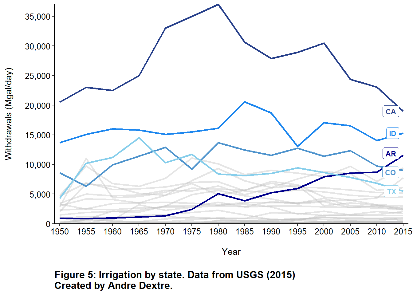
Water Use by State: Public Supply vs Irrigation
The most populous states such as California, Texas, New York, Florida, and Illinois are the biggest water users For public supply in the US. Additionally, for irrigation the biggest water users are western states that tend to have dry climates and depend on groundwater supply for irrigation.
#Create new object for years 1965 to 2015
#SW is ps, ir/it, do, ls/li, oi/in/mi/pt
source_wu_1965 <- d_wu_1965 %>%
  mutate(State = area,
         Population = tp_tot_pop,
         SW = ps_wsw_fr + ir_wsw_fr + do_wsw_fr + ls_wsw_fr +
           oi_wsw_fr + pt_wsw_fr,
         GW = ps_wgw_fr + ir_wgw_fr + do_wgw_fr + + ls_wgw_fr +
           oi_wgw_fr + pt_wgw_fr,
         Total = SW + GW,
         Year = 1965) %>%
  select(State, Year, Total, GW, SW, Population) %>%
  pivot_longer(3:5, names_to = "Source", values_to = "Withdrawals")

#1970
source_wu_1970 <- d_wu_1970 %>%
  mutate(State = area,
         Population = tp_tot_pop,
         SW = ps_wsw_fr + ir_wsw_fr + do_wsw_fr + ls_wsw_fr +
           oi_wsw_fr + pt_wsw_fr,
         GW = ps_wgw_fr + ir_wgw_fr + do_wgw_fr + + ls_wgw_fr +
           oi_wgw_fr + pt_wgw_fr,
         Total = SW + GW,
         Year = 1970) %>%
  select(State, Year, Total, GW, SW, Population) %>%
  pivot_longer(3:5, names_to = "Source", values_to = "Withdrawals")

#1975
source_wu_1975 <- d_wu_1975 %>%
  mutate(State = area,
         Population = tp_tot_pop,
         SW = ps_wsw_fr + ir_wsw_fr + do_wsw_fr + ls_wsw_fr +
           oi_wsw_fr + pt_wsw_fr,
         GW = ps_wgw_fr + ir_wgw_fr + do_wgw_fr + + ls_wgw_fr +
           oi_wgw_fr + pt_wgw_fr,
         Total = SW + GW,
         Year = 1975) %>%
  select(State, Year, Total, SW, GW, Population) %>%
  pivot_longer(3:5, names_to = "Source", values_to = "Withdrawals")

#1980
source_wu_1980 <- d_wu_1980 %>%
  mutate(State = area,
         Population = tp_tot_pop,
         SW = ps_wsw_fr + ir_wsw_fr + do_wsw_fr + ls_wsw_fr +
           oi_wsw_fr + pt_wsw_fr,
         GW = ps_wgw_fr + ir_wgw_fr + do_wgw_fr + + ls_wgw_fr +
           oi_wgw_fr + pt_wgw_fr,
         Total = SW + GW,
         Year = 1980) %>%
  select(State, Year, Total, GW, SW, Population) %>%
  pivot_longer(3:5, names_to = "Source", values_to = "Withdrawals")

#From 1985 and on add the following:
#Group by state
#Add across columns 1:5
#Add "Year" column

#1985
source_wu_1985 <- d_wu_1985 %>%
  mutate(State = scode,
         Population = po_total,
         SW = ps_wswfr + ir_wswfr + do_ssswf + ls_swtot + in_wswfr +
           mi_wswfr + pt_wswfr,
         GW = ps_wgwfr + ir_wgwfr + do_ssgwf + ls_gwtot + in_wgwfr +
           mi_wgwfr + pt_wgwfr,
         Total = SW + GW,
         Year = 1985) %>%
  select(State, Population, SW, GW, Total, Year) %>%
  group_by(State) %>%
  summarize(across(1:5, sum)) %>%
  pivot_longer(3:5, names_to = "Source", values_to = "Withdrawals") %>%
  mutate(Year = 1985)

#1990
source_wu_1990 <- d_wu_1990 %>%
  mutate(State = scode,
         Population = po_total,
         SW = ps_wswfr + ir_wswfr + ls_swtot + do_ssswf + in_wswfr +
           mi_wswfr + pt_wswfr,
         GW = ps_wgwfr + ir_wgwfr + do_ssgwf + ls_gwtot + in_wgwfr +
           mi_wgwfr + pt_wgwfr,
         Total = SW + GW,
         Year = 1990) %>%
  select(State, Population, SW, GW, Total, Year) %>%
  group_by(State) %>%
  summarise(across(1:5, sum)) %>%
  mutate(Year = 1990) %>%
  pivot_longer(3:5, names_to = "Source", values_to = "Withdrawals")

#1995
source_wu_1995 <- d_wu_1995 %>%
  mutate(State = state_code,
         Population = total_pop,
         SW = ps_wsw_fr + ir_wsw_fr + ls_wsw_fr + do_wsw_fr + in_wsw_fr +
           mi_wsw_fr + pt_wsw_fr,
         GW = ps_wgw_fr + ir_wgw_fr + do_wgw_fr + ls_wgw_fr + in_wgw_fr +
           mi_wgw_fr + pt_wgw_fr,
         Total = SW + GW,
         Year = 1995) %>%
  select(State, Population, SW, GW, Total, Year) %>%
  group_by(State) %>%
  summarize(across(1:5, sum)) %>%
  mutate(Year = 1995) %>%
  pivot_longer(3:5, names_to = "Source", values_to = "Withdrawals")

#2000
source_wu_2000 <- d_wu_2000 %>%
  mutate(State = statefips,
         Population = tp_tot_pop,
         SW = ps_wsw_fr + it_wsw_fr + ls_wsw_fr + do_wsw_fr + mi_wsw_fr +
           in_wsw_fr + pt_wsw_fr,
         GW = ps_wgw_fr + it_wgw_fr + do_wgw_fr + ls_wgw_fr + in_wgw_fr +
           mi_wgw_fr + pt_wgw_fr,
         Total = SW + GW,
         Year = 2000) %>%
  select(State, Population, SW, GW, Total, Year) %>%
  group_by(State) %>%
  summarize(across(1:5, sum)) %>%
  mutate(Year = 2000) %>%
  pivot_longer(3:5, names_to = "Source", values_to = "Withdrawals")

#2005
source_wu_2005 <- d_wu_2005 %>%
  mutate(State = statefips,
         Population = tp_tot_pop,
         SW = ps_wsw_fr + ir_wsw_fr + ls_wsw_fr + do_wsw_fr + in_wsw_fr +
           mi_wsw_fr + pt_wsw_fr,
         GW = ps_wgw_fr + ir_wgw_fr + do_wgw_fr + ls_wgw_fr + in_wgw_fr +
           mi_wgw_fr + pt_wgw_fr,
         Total = SW + GW,
         Year = 2005) %>%
  select(State, Population, SW, GW, Total, Year) %>%
  group_by(State) %>%
  summarize(across(1:5, sum)) %>%
  mutate(Year = 2005) %>%
  pivot_longer(3:5, names_to = "Source", values_to = "Withdrawals")

#2010
source_wu_2010 <- d_wu_2010 %>%
  mutate(State = statefips,
         Population = tp_tot_pop,
         SW = ps_wsw_fr + ir_wsw_fr + li_wsw_fr + do_wsw_fr + mi_wsw_fr +
           in_wsw_fr + pt_wsw_fr,
         GW = ps_wgw_fr + ir_wgw_fr + do_wgw_fr + li_wgw_fr + in_wgw_fr +
           mi_wgw_fr + pt_wgw_fr,
         Total = SW + GW,
         Year = 2010) %>%
  select(State, Population, SW, GW, Total, Year) %>%
  group_by(State) %>%
  summarise(across(1:5, sum)) %>%
  mutate(Year = 2010) %>%
  pivot_longer(3:5, names_to = "Source", values_to = "Withdrawals")

#2015
source_wu_2015 <- d_wu_2015 %>%
  mutate(State = statefips,
         Population = tp_tot_pop,
         SW = ps_wsw_fr + ir_wsw_fr + li_wsw_fr + do_wsw_fr + in_wsw_fr +
           mi_wsw_fr + pt_wsw_fr,
         GW = ps_wgw_fr + ir_wgw_fr + do_wgw_fr + li_wgw_fr + in_wgw_fr +
           mi_wgw_fr + pt_wgw_fr,
         Total = SW + GW,
         Year = 2015) %>%
  select(State, Population, SW, GW, Total, Year) %>%
  group_by(State) %>%
  summarise(across(1:5, sum)) %>%
  mutate(Year = 2015) %>%
  pivot_longer(3:5, names_to = "Source", values_to = "Withdrawals")

#Combine all data frames
wu_all_source <- rbind(source_wu_1965, source_wu_1970, source_wu_1975, source_wu_1980,
                       source_wu_1985, source_wu_1990, source_wu_1995,
                       source_wu_2000, source_wu_2005, source_wu_2010, source_wu_2015) %>%
  filter(State != "78",
         State != "72",
         State != "69",
         State != "66",
         State != "60",
         State != "0",
         State != "11")

#Now do population
population <- wu_all_source %>%
  filter(Source == "GW") %>%
  select(-Source, -Withdrawals) %>%
  group_by(Year) %>%
  summarize(across(Population, sum))

#Create source
source <- wu_all_source %>%
  select(Source, Year, Withdrawals, State) %>%
  group_by(Year, Source) %>%
  summarize(across(Withdrawals, sum))

#Create plot
ggplot() +
  #The columns for sectors seem to be stack onto top of one another for each year
  geom_col(data = source, aes(x = Year, y = Withdrawals,
                              fill = reorder(Source, Withdrawals)),
           stat = "identity",
           color = "black",
           #To put the columns side by side, we use the position_doge and width argument
           width = 4, position = position_dodge(3.5)) +
  scale_fill_manual(values = c("lightsteelblue", "deepskyblue", "midnightblue")) +
  #Create population line (pink)
  geom_line(data = population, aes(x = Year, y = Population, col = "Population"),
            size = 2) +
  #Adds legend and color
  scale_color_manual(values = c("deeppink")) +
  #Add highlight on the line plot
  #Add Labels
  labs(x = "Year",
       y = "Withdrawals (Mgal/day)\n",
       caption = "Figure 6: Trends in population and freshwater withdrawals by source in USA.\nData from USGS (1965 - 2015)",
       fill = "") +
  #Get rid of grid lines and makes the graph easier to read
  theme_few() +
  #Add theme and edit
  theme(axis.text = element_text(color = "black", size = 8),
        axis.ticks.x = element_line(color = "black"),
        axis.ticks.y = element_line(color = "black"),
        plot.caption = element_text(hjust = 0, size = 10, face = "bold"),
        legend.position = "top",
        legend.title = element_blank(),
        axis.title.x = element_text(color = "black", size = 10),
        axis.title.y = element_text(color = "black", size = 10),
        axis.title.y.right = element_text(color = "deeppink", size = 10),
        axis.text.y.right = element_text(color = "deeppink"),
        text = element_text(size = 10)) +
  scale_x_continuous(breaks = scales::pretty_breaks(n = 14)) +
  scale_y_continuous(breaks = scales::pretty_breaks(n = 10),
                     limits = c(0, 400000),
                     label = label_comma(),
                     expand = c(0, 0),
                     sec.axis = sec_axis(trans = ~./1000,
                                         breaks = scales::pretty_breaks(n = 9),
                                         name = "Population (Millions)\n",
                                         label = label_comma()))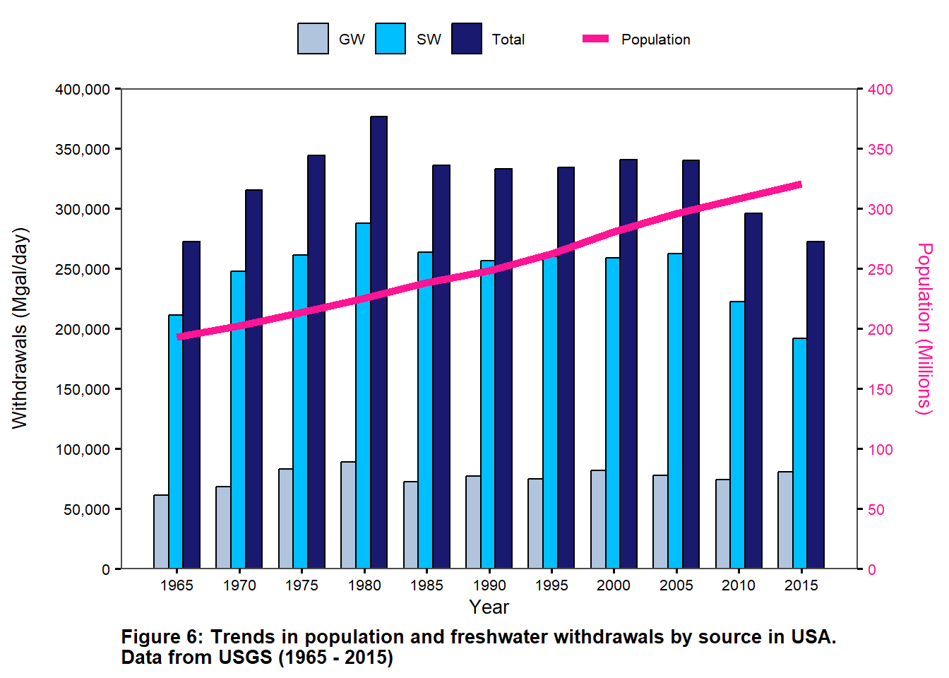
Freshwater Withdrawals by Source in the USA: Groundwater vs Surface Water (1965-2015)
Total Freshwater withdrawals had a steady increase from 1965 until it peaked in 1980. After 1985, total freshwater withdrawals decreased and plateaued from 1985 until 2005, where it continued to decreased. Freshwater withdrawals from surface water makes up most of the total freshwater withdrawals in the US. Fresh water withdrawals from groundwater saw a slight increased from 1965-1980, but it remained low in the following years compared to surface water freshwater withdrawals.
Total Freshwater Withdrawals and Population Trends in the USA (1965-2015) From 1965 to 1980, there is a positive correlation between an increasing population and total freshwater withdrawals. In 1985, total freshwater withdrawals started to decrease while population was still growing. Additionally, from 2005-2015, as population increased, total freshwater withdrawals decreased, this is likely due to more water conservation practices after the 1980s and water use reductions due to extreme drought in the American West.
wu_co_source <- wu_all_source %>%
  filter(State == 8)
source_co <- wu_co_source %>%
  select(Source, Year, Withdrawals, State) %>%
  group_by(Year, Source) %>%
  summarize(across(Withdrawals, sum))

population_co <- wu_co_source %>%
  filter(Source == "GW") %>%
  select(-Source, -Withdrawals) %>%
  group_by(Year) %>%
  summarize(across(Population, sum))

ggplot() +
  geom_col(data = source_co, aes(x = Year, y = Withdrawals,
                                 fill = reorder(Source, Withdrawals)),
           stat = "identity",
           color = "black",
           width = 4,
           position = position_dodge(3.5)) +
  scale_fill_manual(values = c("lightsteelblue", "deepskyblue", "midnightblue")) +
  #Creates a ggplot with pink line
  geom_line(data = population_co, aes(x = Year, y = Population*2, col = "Population"),
            size = 2) +
  scale_color_manual(values = c("deeppink")) +
  #adds labels on x and y axis as well as a figure caption
  labs(x = "Year",
       y = "Withdrawals (Mgal/day)\n",
       caption = "Figure 7: Trends in population and fresh water withdrawals by source in CO.
Data from USGS (1965 - 2015)",
fill = "") +
  #this code got rid of grid lines in the background
  #and makes the graph easier to read
  theme_few() +
  #One piece of code not outlined here is axis.ticks.y and .x = element_line which adds in the axis tick#I implemented the code as follows:
  theme(axis.text = element_text(color = "black", size = 8),
        axis.ticks.x = element_line(color = "black"),
        axis.ticks.y = element_line(color = "black"),
        plot.caption = element_text(hjust = 0, size = 10, face = "bold"),
        legend.position = "top",
        legend.title = element_blank(),
        axis.title.x = element_text(color = "black", size = 10),
        axis.title.y = element_text(color = "black", size = 10),
        axis.title.y.right = element_text(color = "deeppink", size = 10),
        axis.text.y.right = element_text(color = "deeppink"),
        text = element_text(size = 10)) +
  #puts more years on the x-axis
  scale_x_continuous(breaks = scales::pretty_breaks(n=14)) +
  #puts more withdrawal numbers on the y axis between the numbers 0 and 2000000
  #the trans argument is multiplying by two because we need a way to represent
  #the data that has been manipulated by dividing by two. This way the data can
  #remain within the graph and still represent the real values of withdrawals.
  scale_y_continuous(breaks = scales::pretty_breaks(n = 10),
                     limits = c(0, 16000),
                     label = label_comma(),
                     #the expand code gets rid of the space between column bars and the x-axis
                     expand = c(0,0),
                     sec.axis = sec_axis(trans = ~./2,
                                         breaks = scales::pretty_breaks(n = 9),
                                         name = "Population (Millions)\n",
                                         label = label_comma()))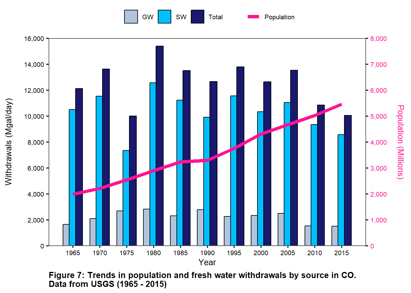
Freshwater Withdrawals by Source in Colorado: Groundwater vs Surface Water (1965-2015) From 1965-2015, the biggest water source for freshwater withdrawals is surface water. From 1965-1970, there was an increased in freshwater withdrawals from both surface water and groundwater. Additionally, there was a huge decrease in surface water withdrawals in 1975, however there was an increase in groundwater withdrawals as well, which was followed by a huge spike in fresh water withdrawal in 1980.From 1985-2005, freshwater withdrawals from surface water and groundwater showed decreased in surface water withdrawals compared to its 1980 peak. After 2005, both surface water and groundwater freshwater withdrawals decreased, most likely due to conservation practices during times of drought.
Total Freshwater Withdrawals and Population Trends in Colorado (1965-2015) Generally, from 1965-1980, as population increased so did total freshwater withdrawals. Additionally, in 1985 and 1990, there was a slight dip in population correlates to a dip in total freshwater withdrawals in Colorado. From 1995-2005, there has been a positive correlation between population and freshwater withdrawals. However, from 2010 and onward, as population increased, total freshwater withdrawals has decreased. This decrease may correspond to water conservation practices during drought periods in Colorado.
Total Freshwater Withdrawals and Population Trends: Colorado vs USA (1965-2015) One common similarity between the USA plot and Colorado plot, is that the biggest source for freshwater withdrawals is surface water. Another similarity between the two plots is that total freshwater withdrawals peaked in 1980. Additionally, another pattern between both plots is that even though population kept increasing after 2005, total freshwater withdrawals started to decreased. One major difference between the USA plot and Colorado plot is that US total freshwater withdrawals generally increased from 1965 until 1980 and then decreased in the following years. Whereas, Colorado’s total freshwater withdrawals had increases and dips in total freshwater withdrawals from 1965-2015. Another major difference, is that the USA held a steady increase in population throughout 1965-1985, whereas Colorado did see an increasing population, however it did not held a constant increase due to a slight decline in population in 1990.
Irrigation Methods:
Flood: Water is applied freely and distributed over the soil surface by gravity.
Sprinkler: Applies water in a controlled manner in a way similar to rainfall.
Micro-irrigation: Allows water to slowly drip to roots of plants, water is placed directly into the root zone to minimize evaporation.
@online{dextre2022,
  author = {Andre Dextre},
  title = {United {States’} {Water-Use} {Data} {Portfolio} (1950-2015)},
  date = {2022-12-09},
  url = {https://github.com/andredextre/Water_Portfolio},
  langid = {en}
}